Concave and Convex Mirrors

Objective: Explore the images formed by convex and concave mirrors.

Equipment:

• Convex mirror
• Concave mirror
• An object
• Ruler

Procedure:

     convex mirror- A marker was placed in front of the convex mirror.The image appears smaller than the actual object but the object is upright. The image seems further from the mirror then the actual object.        With a ruler placed normal to the mirror's center  we held the mirror a distance d0=0.50m. The height of the marker (our object) was h0=0.12m. Measuring (on the mirror) the size of the image of the marker gave us hi=0.067m when the object is moved closer the image appears bigger and it gets smaller as it moves away.

     concave mirrors- the object was now placed in front of a convex mirror. The object appeared inverted and larger. When the object moved closer it appears upright, and still magnified. The image also appears closer to the mirror then the actual object. Using the ruler  we again placed it 0.50m from the center and we observed an inverted height of 0.21m.

Analysis: This phenomenon can be explained by using a diagram of light rays being reflected off the pen.

 For the convex mirror you see that the point where these rays intersect is where the top of the marker's image appears and this agrees with our observation

For the concave mirror we see the focus and center of the sphere is outside of the mirror. Using the rays it can be seen that the object appears to be inverted which also agrees with our observation.

From this it can be concluded that the image size and orientation depend on the focus or center of the spherical mirror.

Introduction to Reflection and Refraction

Objective: To find a relationship between the angle that the light enters a medium and the angle at which the light is refracted (changed) by traveling through the medium.

Equipment:

• Light box or Laser
• Semicircular plastic or glass prism
• circular protractor (or some way of measuring the incident and refracted angles)

Procedure:
     Part I Set up the beam of light so that it enters at the center of the flat edge of the semicircle. At this point the circular protractor should be under the semicircle and the light should be normal to the edge of the circle.

 Keeping the semicircle and protractor together turn the semicircle by a few degrees and record the values of the angle of incidence and the angle of refraction until you get to 70 degrees .Then graph the angles versus each other and the sin of the angles versus each other.






     Part II Now set up the same system but have the light hit the curved edge as shown below but with the straight edge normal to the incident angle.

Do the same procedure as part one and stop once you cannot see the refracted rays. Graph the  relationships of the angles and graph their sines.

Predictions:
     Part I When the angle of incidence is 0 the light will not be refracted. This experiment will revolve around light traveling from the plastic to air.
     Part II When you begin and the angle of incidence is zero so will the angle of refraction because the light won't bend it it is just traveling straight. When the light hits the flat surface at an angle it will refract more drastically because the angle with the normal will be increasing.

Data:
     Part I

theta 1	theta 2	sin 1	sin 2
0	0	0.0000	0.0000
7	3.5	0.1219	0.0610
10	5	0.1736	0.0872
15	7	0.2588	0.1219
20	12.5	0.3420	0.2164
30	19	0.5000	0.3256
40	26	0.6428	0.4384
50	31	0.7660	0.5150
60	34	0.8660	0.5592
70	39	0.9397	0.6293

      Part II

theta 1	theta 2	sin 1	sin 2
0	0	0.00000	0.00000
5	9	0.08716	0.15643
10	17	0.17365	0.29237
15	25.5	0.25882	0.43051
20	35	0.34202	0.57358
25	45	0.42262	0.70711
30	50	0.50000	0.76604
35	63	0.57358	0.89101
40	83	0.64279	0.99255

Data Analysis: The slopes from the graphs of the sine functions show a ratio of velocities also called an index of refraction. The index of refration for part 1 was 1.45 while for part two it was 1.58. For part 2. 10 trials were not able to be completed. The light stopped being refracted around 40 degrees and was completely reflected. It can be seen from the graph that the angle of refraction was increasing rapidly and eventually moved to the point where it refracted along the side of the object (at the critical angle). The two indexes of refraction from part one and part two are nearly identical and this is because this has to do with the material in which light travels. Therefore, it should be about the same. Any error arose from measuring the angles because the light spanned over multiple degrees.

 As a side note during the experiment there were many points where reflection and refraction occurred together.

Speed of Sound Test

Objective: Verify the speed of sound.

Equipment:

• Logger Pro with Microphone
• Computer
• Long Tube
• Meter Stick

Set Up: The tube was set standing up with the Logger Pro microphone at the top of the tube.

Procedure: The length of the tube was measured with the meter stick to be 0.9643 ± 0.0010 m. A quick sound ( a snap) was made at the top of the tube next to the microphone while data was being recorded. These were the results:
     This was the graph of sound (via pressure sensors) the two significant pieces of data shown are from the initial snap and the echo from the resonating tube. The time from the beginning of the first snap to the beginning of the echo was recorded by taking the difference in time from the first peak of the snap to the first peak of the echo. This was recorded to be 0.00580 ± 0.00005s.

     The speed of sound can be found by dividing the length traveled (two times the length of the tube) by the time it took to travel (found with the echo). 

The speed of sound was recorded to be 332 ± 3.6 m/s. It was important  to make the initial sound a quick as possible as to not interfere with the echo. This can be compared to the value of the speed of sound depending on temperature in the following way.

     This is a reasonable error which could have come from the time we used for the time traveled. The exact points were difficult to determine. This would have been the biggest source of error.

Introduction to Sound

Objective: Explore sound waves.

Equipment:

• Logger Pro with Microphone
• Computer
• Tuning fork

 We set up logger Pro with a microphone to record sound.

To get a sample we made noise into the speaker (saying "aaaaaaaaaa") and set the ample rate high and the sample time very low ( about 0.5 seconds)

In order to study this sample more closely we zoomed in on a portion of the data.

Examining this graph it is obvious that it is not sinusoidal but it is periodic (it repeats after a certain amount of time)
     We estimated about 23 waves in this sample. We did this by counting the peaks in the duration of time. This was difficult because the sample time was very quick like the way an hour can pass in the blink of an eye when your doing a difficult physics problem.
     We measured the period by taking the difference in time recorded between two adjacent peaks. This came out to be 0.00123 seconds. Since frequency is the inverse of period the frequency was shown to be 813 Hz.

     Using the above calculations (and assuming the speed of sound to be 340 meters per second) the wavelength is 0.418 m. To find the amplitude we used two adjacent peaks and found the maximum and minimum and took the average. This came out to be 0.384 m. If we were to get a longer sample the data would be the same some values might vary slightly simple because the sample would give us more to work with so we might be able to get a more accurate average of values.
     This was repeated with my lab partner speaking into the microphone. His values were different he had a lower frequency which led to a shorter wavelengrh but the data was very similar. This is the second data set:

     We then used a tuning fork and recorded the sound on Logger Pro. We struck the fork on the sole of a shoe as to not damage the fork The result was a very smooth looking sinusoidal wave.
     Using the same methods as before the following data was collected.

• Period: 0.00994 s
• Frequency: 101 Hz
•  Wavelength: 3.38 m
• Amplitude: 4.55 cm

To test what would happen if the fork was struck with different intensity we ran a second trial with the tuning fork. We had predicted it would only change the amplitude.
   

 The fork was struck again as to resonate with a different amplitude and this was the result:

• Period: 0.00982 s
• Frequency: 102 Hz
• Wavelength: 3.34 m
• Amplitude: 2.00 cm

    The prediction was correct all the data (excluding the amplitude) was off by an amount of a few figures on the order of the smallest significant figure (experimental error) with the exception of the amplitude.

Standing Waves Experiment

Objective: Understand driven standing waves and investigate resonant conditions for a standing wave.

Equipment:

• Pasco Student Function Generator 
• Pasco Varible Frequency Wave Driver with String
• 50g weight hanger and slotted weight set
• 2 table clamps
• a Pulley 
• Short Rod
• Pendulum clamp
• 2 meter stick

Procedure: The length and mass of the string were measured in order to find the density μ. M=0.00409kg, l=4.43m,so μ=mass per unit length=0.000923(kg/m). Then the system was set up. The string was held in two places on the table, one of which had a mass hung on it (0.250kg) and went over the edge of the table via a pulley. The wave driver was attached to the string 2.00 ±0.02m away from the pulley. The wave driver was hooked up to the function generator. The set up looked like this:

The frequency of the generator was set to make the wave be in the fundamental mode. Then the number of nodes,the oscillation frequency, and the wavelength were recorded.





The frequency was increased to get different harmonics and that information was recorded again.

Harmonic	nodes	λ, m	frequency, Hz
1	2	4	12.1
2	3	2	23.7
3	4	1.333333333	34.3
4	5	1	46.3
5	6	0.8	57.5
6	7	0.666666667	68.9
7	8	0.571428571	80.2
8	9	0.5	90.6
9	10	0.444444444	103.8
10	11	0.4	115.4

     Then the tension was changed by changing the hanging mass(to 0.050kg) and the data was recorded again.

Harmonic	nodes	λ, m	frequency, Hz
1	2	4	4.7
2	3	2	10.3
3	4	1.333333333	15.6
4	5	1	20.9
5	6	0.8	26.3
6	7	0.666666667	31.3
7	8	0.571428571	36.7
8	9	0.5	41.6
9	10	0.444444444	46.7
10	11	0.4	51.5

Data Analysis:
     For the first case Microsoft Excel was used to make a graph of frequency vs. the inverse of wavelength (λ).The slope is also the speed of wave propagation which came out to be 45.697(m/s). The speed of propagation can also be found in the following way:

This gave a wave speed of 51.5(m/s) which is very close to the experimental. In fact it gives an error of 12%.

The same was done for the second case where the mass was changed. The experimental value was 20.81 (given from the graph). Then we can use the same method to find the wave speed theoretically which was 23.0(m/s). The percent error here is 10%

The ratio of the experimental speeds for case one and case two is 2.20. When This is compared to the ratio of the calculated values of the wave speeds (which is 20.24) it is evident that the ratios of the two are nearly identical.

For case one when the ratio of the first and second harmonic frequencies is taken it comes to be 1.96 which is nearly double as it should be to follow the pattern f=nf0 where n is the harmonic number. The same follows for case two where the ratios of the first two harmonic frequencies is 2.19.

Error: There was small error in the measurement of the mass and length of the rope that carried through the experiment. Another source of error came from finding the resonant frequencies. At some points (especially the higher harmonics) it was difficult to pinpoint the exact frequency that gave it the greatest amplitude. The values for the experimental wave speeds determined from the slopes of the graphs were very accurate and gave a r-squared value of 0.9997 so for the most point the experimental frequencies followed the pattern.

Wavelength and Frequency of a Wave Dependence

Fluid Dynamics Lab

Objective: Use Bernoulli equation to figure out the time it takes to drain an amount of water from a bucket with a hole in the bottom and use this to examine experimental error.

Equipment:

• A bucket with a small hole drilled into the side
• Tap water
• Graduated cylinder
• Ruler 
• Stopwatch

Bernoulli"s equation work:

To find the time to empty a volume of water we need to find the rate of flow.

Set up:
First the bucket's hole was taped over. Then the bucket was filled with water and the water level in the bucket was measured with the ruler.

Procedure:
 To get  an idea of the procedure a pilot test was run. The tape was peeled off as the timer was started and the drained water was caught in the graduated cylinder. Once the graduated cylinder was filled to 100 mL then the stopwatch was stopped and the drain hole was covered. Our Pilot run had a time of 
5.23 (+/-) 0.10 s. 

Six official trials were run with the results as listed below. The measurements of the radius of the drain hole and height of the water in the bucket are also listed.

Run	1	2	3	4	5	6
Time to empty (tactual),s ±0.10	5.83	6.35	6.43	6.23	6.04	6.3
Diameter of Drain Hole,  mm	5.8±0.2
Height of Water, cm	15.0±0.2

     Some calculations with the measured values showed that the time to drain the water should have been 2.21s

     Since this is drastically different then the times recorded during the experiment, the equation was rewritten to find the radius of the drain hole needed to empty the same amount of water in the calculated time.

This radius of 3.5mm was different from the measured 5.8mm. This is most likely due to the fact that the calculated 2.2s came from measurements with their own uncertainties. The one measured with a caliper had the direct uncertainty of measurement while the time uncertainty was dependent on 3 other measurements. Since both values of the radius of the drain hole came from measurements the best way to calculate the percent error is as follows.

    The diameter of the whole was said to be a quarter inch (6.35 mm). Comparing this to the measured 5.8±0.2mm gives an error of 9.1% error using the above method.

    The reason this method is used here instead of the %error where the difference is divided by the "True" value is because there is no real True value since both methods depend on measurements with uncertainty.

Fluid Statics Lab

During this "Fluid Statics" lab the objective was to find the Buoyant Force experimentally using various methods and compare the results.

Equipment needed:

• Force Probe 
• Logger Pro 
• String 
• Graduated Cylinder 
• Bucket (to catch overflow) 
• Metal cylinders with hooks 
• Vernier caliper or micrometer caliper 

A. Underwater Weighing Method

This method measures the buoyant force by taking the difference of the weight of the cylinder in the air and in the water.
The force probe was connected to Logger Pro and mounted on a ring stand. The Force probe was then attached to some known weights (via string) in order to calibrate the sensor. Finally the metal cylinder was attached to the force probe.



The force of the tension was taken and recorded to be 1.09 ± 0.01 N. This is also the measure of the weight of the metal cylinder since the system was in equilibrium. Then the graduated cylinder was nearly filled with water and the metal calendar was placed inside while still attached to the system.

The new reading of the tension was 0.69 ± 0.02 N.




The Buoyant Force was 0.40 N ± 0.03.


B. Displaced Fluid Method

The Displaced Fluid Method measures the buoyant force by finding the weight of the water displaced

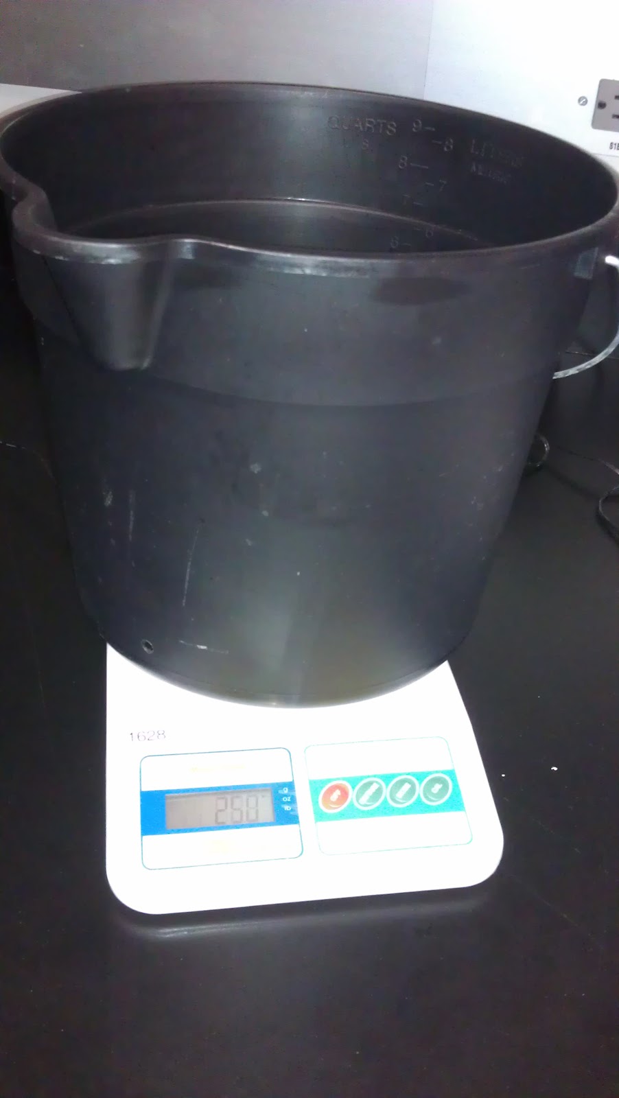
The mass of the bucket was measured to be 0.252 kg ± 0.001.

The graduated cylinder was then filled with water and placed in the bucket. The metal cylinder was placed in the graduated cylinder and a volume of water overflowed from the graduated cylinder equal to the volume of the metal cylinder.




The cylinders were removed from the bucket and the mass of the bucket with the overflow water was taken. It was 0.289 kg ± 0.001.




By Archimedes principle the weight of the displaced water and the buoyant force is 0.363 N ± 0.020.


C. Volume of Object Method

With the Volume of Object Method you fine the volume of the object and with the density of the liquid you are able to find the weight of the water displaced (similar to the previous one).



The metal cylinders dimensions were taken with a micrometer caliper and were as follows:

height: 0.0762± 0.00005m Diameter: 0.0253± 0.00005m



Using the dimensions to find the volume and using the known density of water and acceleration due to gravity the buoyant force was found to be 0.375 N ± 0.018.

Conclusions:

All the values were consistent within the uncertainty. For the first method the uncertainty could have come from measuring the tension in water. The graduated cylinder was a tight fit and if the metal cylinder was touching the sides of the graduated cylinder then it could have given a higher reading for the buoyant force. The second method would have had a lot of uncertainty from the mass of the water. The outside of the graduated cylinder retained some of the water and that wasn't accounted for. The cylinder may also not have been filled to the exact top with water. This would result in a lower buoyant force. In the third part error arose from the fact that the hook on the metal cylinder was no accounted for in the displaced volume. All of these methods were, however, consistent within reasonable error.

I believe that the first method was most accurate because there was less room for error where as the other two had obvious error associated with the procedure (the excess water and the unaccounted for hook).

If, in part A the cylinder had been touching the bottom of the container this would have made our experimental buoyant force much greater because there would be a normal force on the metal cylinder. It would have added to what would have been thought of as the buoyant force and made it too high.